Let us continue our discussion!
Recall the scatterplot in Part I below, now with a fitted regression line that best describes a linear relationship between budget and average rating. This is what is enabled by regression analysis. Typically, regression analysis uses a method called ordinary least squares (OLS). OLS fits the line that minimizes the sum of the squared residuals. Each movie in our dataset has a residual, which is its vertical distance from the regression line. Of course, if the observations lie exactly on the line, the residuals are zero.
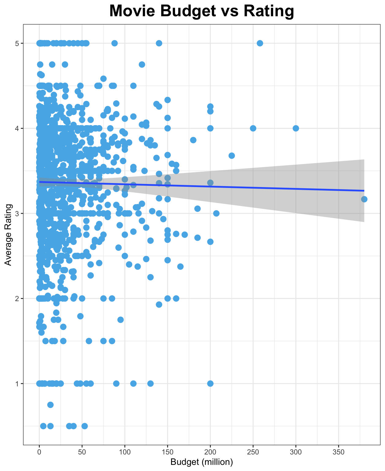
There is an equation describing the regression line that takes the following form: y = a + bx, where a is the y-intercept of the line (the value for y when x = 0) and b is the slope of the line. Then, b represents the “best” linear relationship between budget and average rating for movies in our dataset, as defined by OLS. The variable that is being explained, also known as the dependent variable, denoted as y. The variable that is used to explain the dependent variable is known as explanatory variable or independent variable, denoted as x.
When we run a simple linear regression for our movie data with budget as the explanatory variable and average rating as dependent variable, we get the following results:
average rating = 3.37 – 0.00027*budget
The estimate for b = -0.0027 is known as a regression coefficient or, in our case, the coefficient for the budget. This means that a 1 million increase in budget is associated with a -0.00027 decrease in average rating. But, this equation is not a good representation of the linear relationship between average rating and budget due to i) the correlation coefficient between them is -0.014, very close to zero, and hence exhibit almost no correlation, and ii) the p-value associated with the coefficient on the budget is 0.613, greater than 0.05 or even 0.1, which indicates that this coefficient is not statistically significant – this might be an oversimplification, but we will discuss about p-value later in the future post, just take it for now. In general, it is reasonable to conclude that there is no correlation and causal relationship between budget and average rating.
In a real analytics project, I would not easily say that though – I mean, it would sound like “let us give up on our data”. The good news is that finding a hidden pattern is exciting and, if you were able to reveal it, satisfying. Long story short, let us focus our observation on movies with budgets between $150 – $300 million and with an average rating greater than equal to 2. Now our samples are down to 20 movies. This is not ideal but let me keep going with this for the purpose of demonstration. We see that for this specific group of movies, there is a trend of increase in the average rating as the budget increases. The coefficient correlation is 0.58, which defines a pretty strong positive correlation.

Run a simple linear regression we have the following results:
average rating = 1.20 + 0.0113*budget
So, for the movies with a budget of $150 – 300 million and an average rating of 2 or greater, 1 million increase in budget is associated with a 0.0113 increase in average rating. The p-value of the coefficient for budget is 0.007, which indicates statistical significance of this coefficient.
We revealed one hidden pattern! While, in general, we do not have enough evidence to say that there is a correlation or a causal relationship between budget and average rating, this relationship may exist for certain groups of movies. At least for the 20 movies with budgets ranging from $150 – 300 million and rated 2 or higher, there seems to be a meaningful correlation and causal relationship between their budget and average rating.
Of course we should not stop here. In real analytics projects, we would want to explore further. What are the characteristics of those 20 movies? Maybe they share the same characteristics. What about other movies? Maybe their budget and average rating show a negative correlation or no correlation at all. And so on, and so forth. Anyway, the purpose of “A Semi-Poetic Intro to Statistical Modelling” is to introduce you with the basic statistical modelling: correlation and causation through linear regression. The highlight is that correlation does not imply causation.
Finally, note that linear relationships are not suitable for many real-world problems. As you may already be aware, we do not live in a linear world. Many phenomena are actually non-linear, hence non-linear modelling would be more suitable for such cases. But, that would again be our next topic.
If we choose a group of social phenomena with no antecedent knowledge of the causation or absence of causation among them, then the calculation of correlation coefficients, total or partial, will not advance us a step toward evaluating the importance of the causes at work.
– R. A. Fisher